
Settings#
DataLab provides a comprehensive settings dialog to customize the application behavior, visualization defaults, and I/O operations. The settings are organized into five tabs: General, Processing, Visualization, I/O, and Console.
General#
The General settings tab contains main window and general feature settings:
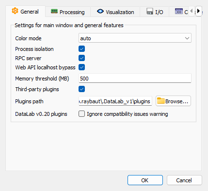
General settings tab#
- Color mode
Choose the color mode for the application interface (e.g., light, dark, or auto).
- Process isolation
When enabled, each computation runs in a separate process, preventing the application from freezing during long computations. This is the recommended setting for better responsiveness.
- RPC server
Enable the RPC (Remote Procedure Call) server to communicate with external applications, such as your own scripts running in Spyder, Jupyter, or other software. This allows programmatic control of DataLab.
- Web API localhost bypass
When enabled (default), connections from localhost (127.0.0.1) to the Web API do not require authentication. This simplifies notebook integration when DataLab-Kernel runs on the same machine. Disable for stricter security if needed.
Note
When this option is enabled, any application running on your local machine can access the DataLab Web API without a token. Disable this option if you need stricter security.
- Memory threshold
Set a threshold (in MB) below which a warning is displayed before loading new data. This helps prevent out-of-memory errors when working with large datasets. Set to 0 to disable the warning.
- Third-party plugins
Enable or disable third-party plugins immediately. Changes are applied without restarting DataLab. When disabled, third-party plugins are not discovered or loaded.
- Plugins path
Specify the directory path where DataLab should look for third-party plugins. DataLab will also discover plugins in your PYTHONPATH. To enable or disable individual plugins, use the
Plugins > Configure plugins...menu action. DataLab then proposes reloading plugins automatically.
Processing#
The Processing settings tab controls computation behavior and default parameters:
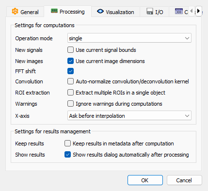
Processing settings tab#
- Operation mode
Choose the operation mode for computations taking N inputs:
Single: single operand mode
Pairwise: pairwise operation mode
Note
These operation modes determine how DataLab handles computations involving multiple objects. They apply to two types of operations:
N→1 operations: Combine N (≥2) objects into 1 output (e.g. sum, average)
N+1→N operations: Apply an operation between N (≥1) objects and 1 operand to produce N outputs (e.g. difference, division)
Single operand mode (default): Operations are applied independently within each group.
For N→1 operations: All objects in each group are combined into one result per group. Example with groups G1={A, B} and G2={C, D}, sum operation:
Result: Σ(A,B) and Σ(C,D) (one per group)
For N+1→N operations: Each selected object is combined with a single reference operand. Example with groups G1={A, B} and G2={C, D}, difference with reference R:
In G1: A-R, B-R
In G2: C-R, D-R
Pairwise operation mode: Objects from different groups are combined at matching positions (all groups must have the same number of objects).
For N→1 operations: Objects at the same position in each group are combined. Example with groups G1={A, B} and G2={C, D}, sum operation:
Result: A+C and B+D (pairing by position)
For N+1→N operations: Objects at matching positions are combined pairwise. Example with groups G1={A, B}, G2={C, D}, difference with group G3={E, F}:
New group 1: A-E, B-F
New group 2: C-E, D-F
- Use signal bounds for new signals
When enabled, the xmin and xmax values for new signals are initialized from the current signal’s bounds. When disabled, default values are used.
- Use image dimensions for new images
When enabled, the width and height values for new images are initialized from the current image’s dimensions. When disabled, default values are used.
- FFT shift
Enable FFT shift to center the zero-frequency component in the frequency spectrum for easier visualization and analysis.
- Extract multiple ROIs in a single object
When enabled, multiple ROIs (Regions of Interest) are extracted into a single object. When disabled, each ROI is extracted into a separate object.
- Ignore warnings
Suppress warning messages during computations.
- X-array compatibility behavior
Choose the behavior when X arrays are incompatible in multi-signal computations:
Ask: display a confirmation dialog (default)
Interpolate: automatically interpolate signals
Result management#
- Keep results in metadata after computation
When enabled, results from previous analyses are kept in the object’s metadata after computation. When disabled, results are removed. This option is disabled by default to avoid confusion from outdated results.
- Show results dialog automatically after processing
When enabled, the results dialog is shown automatically after each processing operation producing results. When disabled, the results dialog is not shown automatically but results can still be viewed using the dedicated button or menu option.
Visualization#
The Visualization settings tab controls how data is displayed. This tab is organized into four sub-tabs: Common, Signals, Images, and Results.
Common settings#
The Common sub-tab contains settings that apply to all visualizations:
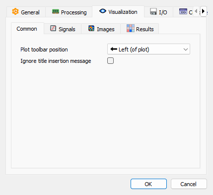
Visualization settings - Common sub-tab#
- Plot toolbar position
Choose where to position the plot toolbar (top, bottom, left, or right of the plot).
- Ignore title insertion message
Suppress the information message when inserting an object title as an annotation label.
Signals#
The Signals sub-tab contains settings specific to signal visualizations:
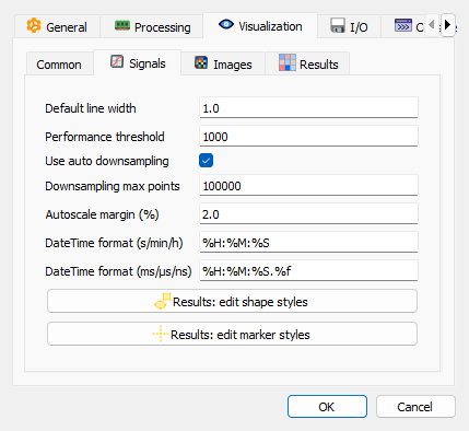
Visualization settings - Signals sub-tab#
- Default line width
Default line width for curves representing signals. This setting affects all signal visualizations unless overridden individually. Note: for signals exceeding the line width performance threshold (see below), the line width is automatically clamped to 1.0 for optimal rendering performance.
- Line width performance threshold
For signals with more than this number of points (default: 1,000), line width is automatically limited to 1.0 for performance reasons. This prevents the ~10x rendering slowdown caused by Qt’s raster engine when drawing thick lines (width > 1.0) on large datasets. For smaller signals, the configured default line width applies normally. This optimization is transparent and requires no user intervention.
- Use auto downsampling
Enable automatic downsampling for large signals to improve performance and visualization clarity.
- Downsampling max points
Maximum number of points to display when downsampling is enabled (default: 10,000).
- Autoscale margin
Percentage of margin to add around data when auto-scaling signal plots. A value of 0.2% adds a small margin for better visualization. Set to 0% for no margin (exact data bounds).
- DateTime format (s/min/h)
Format string for datetime X-axis labels when using standard time units (s, min, h). Uses Python’s strftime format codes (e.g., %H:%M:%S for hours:minutes:seconds).
- DateTime format (ms/μs/ns)
Format string for datetime X-axis labels when using sub-second time units (ms, μs, ns). Uses Python’s strftime format codes (e.g., %H:%M:%S.%f for hours:minutes:seconds.microseconds).
- Results: edit shape styles
Click this button to configure the visual style for annotation shapes (rectangles, circles, segments, etc.) displayed on signal plots. This includes:
Line style, color, and width
Fill pattern, color, and transparency
Symbol shape, size, and colors
These settings apply to all result shapes drawn on signal plots (e.g., peak markers, FWHM indicators, feature detection results).
- Results: edit marker styles
Click this button to configure the visual style for cursor markers on signal plots. This includes:
Line style, color, and width
Symbol appearance
Text label formatting and positioning
Background transparency
These settings apply to cursor-type markers used in signal analysis results.
Images#
The Images sub-tab contains settings specific to image visualizations:
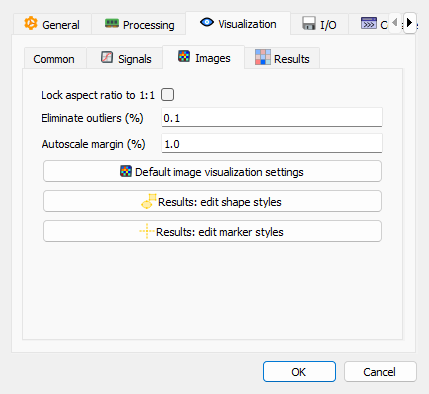
Visualization settings - Images sub-tab#
- Lock aspect ratio to 1:1
When enabled, the aspect ratio of images is locked to 1:1. When disabled, the aspect ratio is determined by the physical pixel size (default and recommended setting).
- Eliminate outliers
Percentage of the highest and lowest values to eliminate from the image histogram. Recommended values are below 1%.
- Autoscale margin
Percentage of margin to add around data when auto-scaling image plots. A value of 0.2% adds a small margin for better visualization. Set to 0% for no margin (exact data bounds).
- Default image visualization settings
Click this button to configure default visualization settings for images (colormap, interpolation, contrast, etc.).
- Results: edit shape styles
Click this button to configure the visual style for annotation shapes displayed on image plots. Parameters are similar to signal shapes but optimized for image visualization (e.g., different colors for better visibility on images).
- Results: edit marker styles
Click this button to configure the visual style for cursor markers on image plots.
Results#
The Results sub-tab contains settings for displaying analysis results on plots:
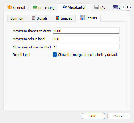
Visualization settings - Results sub-tab#
These settings control how analysis results are displayed on plots to prevent performance issues with large datasets:
- Maximum shapes to draw
Maximum number of geometry shapes to draw on the plot (default: 1,000). When the number of shapes exceeds this limit, only the first N shapes are drawn and a warning label is displayed.
- Maximum cells in label
Maximum number of table cells (rows × columns) to display in merged result labels on plots (default: 100). When the number of cells exceeds this limit, the table is truncated.
- Maximum columns in label
Maximum number of columns to display in merged result labels (default: 15). When the number of columns exceeds this limit, only the first N columns are displayed.
- Show the merged result label by default
When enabled, the merged result label is shown on the plot by default for new objects. This setting can be toggled per-object using the checkbox in the Properties panel.
Note
These settings affect only the visualization of results on plots. They do not affect the actual computation or storage of results in metadata.
I/O#
The I/O settings tab controls input/output operations:
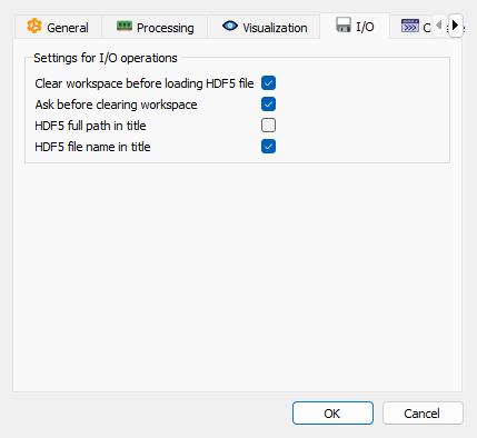
I/O settings tab#
- Clear workspace before loading HDF5 file
When enabled, the workspace is cleared before loading an HDF5 file.
- Ask before clearing workspace
When enabled, a confirmation dialog is displayed before clearing the workspace.
- HDF5 full path in title
When enabled, the full path of the HDF5 dataset is used as the title for the signal/image object. When disabled, only the dataset name is used.
- HDF5 file name in title
When enabled, the HDF5 file name is appended as a suffix to the title of the signal/image object.
Console#
The Console settings tab configures the internal console for debugging and advanced users:
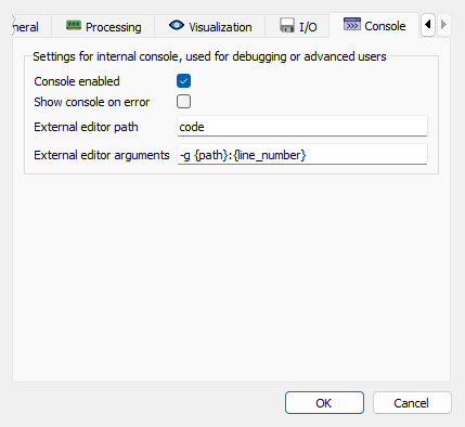
Console settings tab#
- Console enabled
Enable the internal Python console for debugging and advanced scripting.
- Show console on error
When enabled, the console is automatically shown when an error occurs in the application. This is useful for debugging as it allows you to see the error traceback.
- External editor path
Path to an external text editor to use for editing Python code from the console.
- External editor arguments
Command-line arguments to pass to the external editor.