
Operations on Images#
This section describes the operations that can be performed on images.
See also
Processing Images for more information on image processing features, or Analysis features on Images for information on analysis features on images.
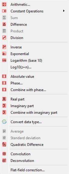
Screenshot of the “Operations” menu.#
When the “Image Panel” is selected, the menus and toolbars are updated to provide image-related actions.
The “Operations” menu allows you to perform various operations on the current image or group of images. It also allows you to extract profiles, distribute images on a grid, or resize images.
Operations with a constant#
Create a new image which is the result of a constant operation on each selected image:
Operation |
Equation |
|---|---|
|
\(z_{k} = z_{k-1} + conv(c)\) |
|
\(z_{k} = z_{k-1} - conv(c)\) |
|
\(z_{k} = conv(z_{k-1} \times c)\) |
|
\(z_{k} = conv(\dfrac{z_{k-1}}{c})\) |
 Add
Add Subtract
 Multiply
 Divide
where \(c\) is the constant value and \(conv\) is the conversion function which handles data type conversion (keeping the same data type as the input image).
Basic arithmetic operations#
Arithmetic operations are performed pixel by pixel between the selected images.
Operation |
Description |
|---|---|
|
\(z_{M} = \sum_{k=0}^{M-1}{z_{k}}\) |
|
\(z_{2} = z_{1} - z_{0}\) |
|
\(z_{M} = \prod_{k=0}^{M-1}{z_{k}}\) |
|
\(z_{2} = \dfrac{z_{1}}{z_{0}}\) |
|
\(z_{2} = \dfrac{1}{z_{1}}\) |
|
\(z_{2} = \exp(z_{1})\) |
|
\(z_{2} = \log_{10}(z_{1})\) |
 Sum
Sum Difference
 Product
 Division
 Inverse
 Exponential
 Logarithm (base 10)
Basic mathematical functions#
Function |
Description |
|---|---|
|
\(z_{k} = \exp(z_{k})\) |
|
\(z_{k} = \log_{10}(z_{k})\) |
Log10(z+10) |
\(z_{k} = \log_{10}(z_{k}+n)\) (useful if image background is zero) |
Convolution and Deconvolution#
Operation |
Implementation |
|---|---|
|
Based on scipy.signal.convolve |
|
Frequency domain deconvolution |
 Convolution
 Deconvolution
Absolute value and complex image operations#
Operation |
Description |
|---|---|
|
\(z_{k} = |z_{k-1}|\) |
|
|
|
Consider current image as the module and allow to select a image
representing the phase to merge them in a complex image
|
|
\(z_{k} = \Re(z_{k-1})\) |
|
\(z_{k} = \Im(z_{k-1})\) |
|
Consider current image as the real part and allow to select a image
representing the imaginary part to merge them in a complex image
|
 Absolute value
 Phase (argument)
 Real part
 Imaginary part
Data type conversion#
The “Convert data type”  action allows you to convert the data type
of the selected images. For integer data types, the conversion is done by clipping
the values to the new data type range before effectively converting the data type.
For floating point data types, the conversion is straightforward.
action allows you to convert the data type
of the selected images. For integer data types, the conversion is done by clipping
the values to the new data type range before effectively converting the data type.
For floating point data types, the conversion is straightforward.
Note
Data type conversion uses the sigima.tools.datatypes.clip_astype()
function which relies on numpy.ndarray.astype() function with
the default parameters (casting=’unsafe’).
Statistics between images#
Create a new image which is the result of a statistical operation on each pixel of the selected images:
Operation |
Description |
|---|---|
|
\(z_{M} = \dfrac{1}{M}\sum_{k=0}^{M-1}{z_{k}}\) |
|
\(z_{M} = \sqrt{\dfrac{1}{M}\sum_{k=0}^{M-1}{(y_{k} - \bar{y})^{2}}}\) |
|
\(z_{2} = \dfrac{z_{1} - z_{0}}{\sqrt{2}}\) |
 Average
 Standard Deviation
 Quadratic difference
Flat-field correction#
Create a new image which is flat-field correction of the two selected images:
where \(z_{0}\) is the raw image, \(z_{f}\) is the flat field image, \(z_{threshold}\) is an adjustable threshold and \(\overline{z_{f}}\) is the flat field image average value:
Note
Raw image and flat field image are supposedly already corrected by performing a dark frame subtraction.