
Processing Signals#
This section describes the signal processing features available in DataLab.
See also
Operations on Signals for more information on operations that can be performed on signals, or Analysis features on Signals for information on analysis features on signals.
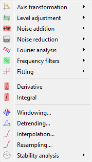
Screenshot of the “Processing” menu.#
When the “Signal Panel” is selected, the menus and toolbars are updated to provide signal-related actions.
The “Processing” menu allows you to perform various processing on the selected signals, such as smoothing, normalization, or interpolation.
Axis transformation#
Linear calibration#
Create a new signal which is a linear calibration of each selected signal with respect to X or Y axis:
Parameter |
Linear calibration |
|---|---|
X-axis |
\(x_{1} = a.x_{0} + b\) |
Y-axis |
\(y_{1} = a.y_{0} + b\) |
Swap X/Y axes#
Create a new signal which is the result of swapping X/Y data.
Reverse X-axis#
Create a new signal which is the result of reversing X data.
Replace X by other signal’s Y#
Create a new signal by combining two signals, using Y values from the second signal as X coordinates for the first signal’s Y values.
This feature is particularly useful for calibration scenarios, such as:
Applying wavelength calibration to spectroscopy data
Using a calibrated reference signal to rescale measurement data
Combining signals where one contains calibration points
The two signals must have the same number of points. The operation directly uses the Y arrays without interpolation.
Input |
Description |
|---|---|
Signal 1 |
Provides the Y data for the output signal |
Signal 2 |
Provides the Y data that becomes the X coordinates of the output signal |
X-Y mode#
Create a new signal by simulating the X-Y mode of an oscilloscope.
This operation plots one signal as a function of another by:
Finding the overlapping X range between both signals
Resampling both signals onto a common X grid within that overlap
Using the resampled Y values as coordinates (first signal’s Y as X, second signal’s Y as Y)
Note
This is different from “Replace X by other signal’s Y” as it performs interpolation to handle signals with different X arrays.
Convert to Cartesian coordinates#
Create a new signal which is the result of converting polar coordinates to Cartesian coordinates.
This function assumes that the x-axis represents the radius and the y-axis the angle.
Warning
A radius cannot be negative. Any negative value is clipped to 0.
Convert to polar coordinates#
Create a new signal which is the result of converting Cartesian coordinates to polar coordinates.
Level adjustment#
Normalize#
Create a new signal which is the normalization of each selected signal by maximum, amplitude, sum, energy or RMS:
Parameter |
Normalization |
|---|---|
Maximum |
\(y_{1}= \dfrac{y_{0}}{\max\left(y_{0}\right)}\) |
Amplitude |
\(y_{1}= \dfrac{y_{0}'}{\max\left(y_{0}'\right)}\) with \(y_{0}'=y_{0}-\min\left(y_{0}\right)\) |
Area |
\(y_{1}= \dfrac{y_{0}}{\sum_{n=0}^{N}y_{0}[n]}\) |
Energy |
\(y_{1}= \dfrac{y_{0}}{\sqrt{\sum_{n=0}^{N}\left|y_{0}[n]\right|^2}}\) |
RMS |
\(y_{1}= \dfrac{y_{0}}{\sqrt{\dfrac{1}{N}\sum_{n=0}^{N}\left|y_{0}[n]\right|^2}}\) |
Clipping#
Create a new signal which is the result of clipping each selected signal.
Offset correction#
Create a new signal which is the result of offset correction of each selected signal. This operation is performed by subtracting the signal baseline which is estimated by the mean value of a user-defined range.
Noise addition#
Generate new signals by adding the same noise to each selected signal. The available noise types are:
Noise |
Description |
|---|---|
Gaussian |
Normal distribution |
Uniform |
Uniform distribution |
Poisson |
Poisson distribution |
Noise reduction#
Create a new signal which is the result of noise reduction of each selected signal.
The following filters are available:
Filter |
Formula/implementation |
|---|---|
Gaussian filter |
|
Moving average |
|
Moving median |
|
Wiener filter |
Fourier analysis#
Zero padding#
Create a new signal which is the result of zero padding of each selected signal.
The following parameters are available:
Parameter |
Description |
|---|---|
Strategy |
Zero padding strategy (see below) |
Number of points |
Custom length (if strategy is “custom”) |
Zero padding strategy refers to the method used to increase the length of the signal, and it can be one of the following:
Strategy |
Description |
|---|---|
next_pow2 |
Next power of 2 (e.g. 1024 → 2048) |
double |
Double the length (e.g. 1024 → 2048) |
triple |
Triple the length (e.g. 1024 → 3072) |
custom |
Custom length (user-defined) |
Frequency filters#
Create a new signal which is the result of applying a frequency filter to each selected signal.
The following filters are available:
Filter |
Description |
|---|---|
|
Filter out high frequencies, above a cutoff frequency |
|
Filter out low frequencies, below a cutoff frequency |
|
Filter out frequencies outside a range |
|
Filter out frequencies inside a range |
 Low-pass
 High-pass
 Band-pass
 Band-stop
For each filter, the following methods are available:
Method |
Description |
|---|---|
Bessel |
Bessel filter, using SciPy’s scipy.signal.bessel function |
Brick wall |
Ideal (rectangular) filter in the frequency domain |
Butterworth |
Butterworth filter, using SciPy’s scipy.signal.butter function |
Chebyshev I |
Chebyshev type I filter, using SciPy’s scipy.signal.cheby1 function |
Chebyshev II |
Chebyshev type II filter, using SciPy’s scipy.signal.cheby2 function |
Elliptic |
Elliptic filter, using SciPy’s scipy.signal.ellip function |
Fitting#
Fit a model to each selected signal. This can be done automatically or through an interactive curve fitting dialog.
Model |
Equation |
|---|---|
Linear |
\(y = c_{0} + c_{1} \cdot x\) |
Polynomial |
\(y = c_{0} + c_{1} \cdot x + c_{2} \cdot x^2 + ... + c_{n} \cdot x^n\) |
Gaussian |
\(y = y_{0} + A \exp\left(-\dfrac{1}{2} \left(\dfrac{x - x_{0}}{\sigma}\right)^2\right)\) |
Lorentzian |
\(y = y_{0} + \dfrac{A}{1+\left(\dfrac{x-x_{0}}{\sigma}\right)^2}\) |
Voigt |
\(y = y_{0} + A \cdot \dfrac{\Re\left(w(z)\right)}{\Re\left(w(j/\sqrt{2})\right)}\) with \(w(z) = \exp(-z^2) \operatorname{erfc}(-jz)\) and \(z = \dfrac{x - x_{0} + j \sigma}{\sqrt{2} \sigma}\) |
Multi-Gaussian |
\(y = y_{0} + \sum_{i=1}^{N} A_{i} \exp\left(-\dfrac{1}{2} \left(\dfrac{x - x_{0,i}}{\sigma_{i}}\right)^2\right)\) |
Multi-Lorentzian |
\(y = y_{0} + \sum_{i=1}^{N} \dfrac{A_{i}}{1 + \left(\dfrac{x - x_{0,i}}{\sigma_{i}}\right)^2}\) |
Planck |
\(y = y_{0} + A \cdot \left(\dfrac{x}{x_{0}}\right)^{-5} \cdot \left(\exp\left(\dfrac{5 x_{0}}{\sigma \cdot x}\right)-1\right)^{-1}\) where \(x_{0}\) and \(\sigma\) are scale and width factors (see the note below) |
Two half Gaussians |
\(y = y_{L} + A_{L} \cdot \exp\left(-\dfrac{1}{2}\left(\dfrac{x - x_{0}}{\sigma_{L}}\right)^2\right)\) if \(x < x_{0}\)
\(y = y_{R} + A_{R} \cdot \exp\left(-\dfrac{1}{2}\left(\dfrac{x - x_{0}}{\sigma_{R}}\right)^2\right)\) otherwise
|
Two back-to-back exponentials |
\(y = y_{0} + A_{L} \cdot \exp\left(B_{L} \cdot x\right)\) if \(x < x_{c}\)
\(y = y_{0} + A_{R} \cdot \exp\left(B_{R} \cdot x\right)\) otherwise
|
Exponential |
\(y = y_{0} + A \exp\left(B \cdot x\right)\) |
Sinusoidal |
\(y = y_{0} + A \sin\left(2 \pi f \cdot x + \phi\right)\) |
Cumulative Distribution Function (CDF) |
\(y = y_{0} + A \erf\left(\dfrac{x - x_{0}}{\sqrt{2} \sigma}\right)\) |
Sigmoid |
\(y = y_{0} + \dfrac{A}{1 + \exp\left(-k \left(x - x_{0}\right)\right)}\) |
For Gaussian, Lorentzian and Voigt models, \(A\) is the signed peak height above the baseline \(y_0\), expressed in the signal’s Y unit.
Note
The Planck model is over-parameterized: it is invariant under \(x_{0} \rightarrow k x_{0}\), \(\sigma \rightarrow k \sigma\), \(A \rightarrow A/k^5\). Only the ratio \(x_{0}/\sigma\) and the product \(A \cdot x_{0}^5\) are determined by the data, so the individual fitted values must not be interpreted on their own. In particular the emission peak is located at approximately \(1.007 \, x_{0}/\sigma\), not at \(x_{0}\).
Multi-peak fit parameters#
For Multi-Gaussian and Multi-Lorentzian fits, the peak-detection dialog first
selects the center \(x_{0,i}\) of each component. These positions remain fixed:
the interactive fit dialog only exposes controls for each amplitude_i and
sigma_i parameter and for the common y0 baseline.
When the fit is accepted, the generated signal stores the complete model under
metadata["fit_params"], including every fixed x0_i center. The metadata may
be inspected with the Metadata button or exported to a JSON .dlabmeta file
using the metadata import/export actions.
The exported parameters are sufficient to evaluate the theoretical model on any X axis outside DataLab:
import numpy as np
from sigima.tools.signal import fitting

fit_params = fitted_signal.metadata["fit_params"]
x = np.linspace(xmin, xmax, size)
y_theoretical = fitting.evaluate_fit(x, **fit_params)
Evaluate fit#
Apply a previously computed fit to a signal. This feature uses the fit parameters stored in the signal metadata (from a prior fitting operation) to generate the fitted curve. This is useful to evaluate the fit on a different X range or on a different signal.
Derivative#
Create a new signal which is the derivative of each selected signal. Based on numpy.gradient.
Integral#
Create a new signal which is the integral of each selected signal. Based on scipy.integrate.cumulative_trapezoid.
Windowing#
Create a new signal which is the result of applying a window function to each selected signal.
The following window functions are available:
Window function |
Reference |
|---|---|
Barthann |
|
Bartlett |
|
Blackman |
|
Blackman-Harris |
|
Bohman |
|
Boxcar (rectangular) |
|
Cosine |
|
Exponential |
|
Flat top |
|
Gaussian |
|
Hamming |
|
Hann |
|
Kaiser |
|
Lanczos |
|
Nuttall |
|
Parzen |
|
Taylor |
|
Tukey |
Detrending#
Create a new signal which is the detrending of each selected signal. This features is based on SciPy’s scipy.signal.detrend function.
The following parameters are available:
Parameter |
Description |
|---|---|
Method |
Detrending method: ‘linear’ or ‘constant’. See SciPy’s scipy.signal.detrend function. |
Interpolation#
Create a new signal which is the interpolation of each selected signal with respect to a second signal X-axis (which might be the same as one of the selected signals).
The following interpolation methods are available:
Method |
Description |
|---|---|
Linear |
Linear interpolation, using using NumPy’s interp function |
Spline |
Cubic spline interpolation, using using SciPy’s scipy.interpolate.splev function |
Quadratic |
Quadratic interpolation, using using NumPy’s polyval function |
Cubic |
Cubic interpolation, using using SciPy’s Akima1DInterpolator class |
Barycentric |
Barycentric interpolation, using using SciPy’s BarycentricInterpolator class |
PCHIP |
Piecewise Cubic Hermite Interpolating Polynomial (PCHIP) interpolation, using using SciPy’s PchipInterpolator class |
Resampling#
Create a new signal which is the resampling of each selected signal.
The following parameters are available:
Parameter |
Description |
|---|---|
Method |
Interpolation method (see previous section) |
Fill value |
Interpolation fill value (see previous section) |
Xmin |
Minimum X value |
Xmax |
Maximum X value |
Mode |
Resampling mode: step size or number of points |
Step size |
Resampling step size |
Number of points |
Resampling number of points |
Stability analysis#
Create a new signal which is the result of a stability analysis of each selected signal.
The following stability analysis methods are available:
Function |
Description |
|---|---|
Allan variance |
Measure of the stability of a signal: defined as the variance of the difference between two successive measurements as a function of the time interval between them. |
Allan deviation |
Square root of the Allan variance. |
Overlapping Allan variance |
A more robust version of the Allan variance that overlaps successive segments to improve statistical confidence. |
Modified Allan variance |
A variation of the Allan variance that accounts for phase noise by introducing a filtering operation. |
Hadamard variance |
An alternative to Allan variance, more robust to linear frequency drift in the signal |
Total variance |
Extends the Allan variance concept to cover all possible averaging intervals. |
Time deviation |
Derived from Allan deviation, quantifies stability in terms of time rather than frequency. |
Note
The “All stability features” option allows to compute all stability analysis methods at once.