Processing Images

This section describes the image processing features available in DataLab.

See also

Operations on Images for more information on operations that can be performed on images, or Analysis features on Images for information on analysis features on images.

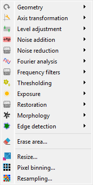
Screenshot of the “Processing” menu.

When the “Image Panel” is selected, the menus and toolbars are updated to provide image-related actions.

The “Processing” menu allows you to perform various processing on the current image or group of images: it allows you to apply filters, to perform exposure correction, to perform denoising, to perform morphological operations, and so on.

Axis transformation

Linear calibration

Create a new image which is a linear calibration of each selected image with respect to Z axis:

Parameter	Linear calibration
Z-axis	\(z_{1} = a.z_{0} + b\)

Swap X/Y axes

Create a new image which is the result of swapping X/Y data.

Level adjustment

Normalize

Create a new image which is the normalized version of each selected image by maximum, amplitude, sum, energy or RMS:

Normalization	Equation
Maximum	\(z_{1} = \dfrac{z_{0}}{z_{max}}\)
Amplitude	\(z_{1} = \dfrac{z_{0}}{z_{max}-z_{min}}\)
Area	\(z_{1} = \dfrac{z_{0}}{\sum_{i=0}^{N-1}{z_{i}}}\)
Energy	\(z_{1}= \dfrac{z_{0}}{\sqrt{\sum_{n=0}^{N}|z_{0}[n]|^2}}\)
RMS	\(z_{1}= \dfrac{z_{0}}{\sqrt{\dfrac{1}{N}\sum_{n=0}^{N}|z_{0}[n]|^2}}\)

Clipping

Apply the clipping to each selected image.

Offset correction

Create a new image which is the result of offset correction on each selected image. This operation is performed by subtracting the image background value which is estimated by the mean value of a user-defined rectangular area.

Noise reduction

Create a new image which is the result of noise reduction on each selected image.

The following filters are available:

Filter	Formula/implementation
Gaussian filter	scipy.ndimage.gaussian_filter
Moving average	scipy.ndimage.uniform_filter
Moving median	scipy.ndimage.median_filter
Wiener filter	scipy.signal.wiener

Fourier analysis

Create a new image which is the result of a Fourier analysis on each selected image.

The following functions are available:

Function	Description	Formula/implementation
FFT	Fast Fourier Transform	numpy.fft.fft2
Inverse FFT	Inverse Fast Fourier Transform	numpy.fft.ifft2
Magnitude spectrum	Optionnal: use logarithmic scale (dB)	\(z_{1} = |FFT(z_{0})|\) or \(z_{1} = 20 \log_{10}(|FFT(z_{0})|)\) (dB)
Phase spectrum		\(z_{1} = \angle(FFT(z_{0}))\)
Power spectral density	Optionnal: use logarithmic scale (dB)	\(z_{1} = |FFT(z_{0})|^2\) or \(z_{1} = 10 \log_{10}(|FFT(z_{0})|^2)\) (dB)

Note

FFT and inverse FFT are performed using frequency shifting if the option is enabled in DataLab settings (see Settings).

Thresholding

Create a new image which is the result of thresholding on each selected image, eventually based on user-defined parameters (“Parametric thresholding”).

The following parameters are available when selecting “Parametric thresholding”:

Parameter	Description
Threshold method	The thresholding method to use (see table below)
Bins	Number of bins for histogram calculation
Value	Threshold value
Operation	Operation to apply (> or <)

The following thresholding methods are available:

Method	Implementation
Manual	Manual thresholding (user-defined parameters)
ISODATA	skimage.filters.threshold_isodata
Li	skimage.filters.threshold_li
Mean	skimage.filters.threshold_mean
Minimum	skimage.filters.threshold_minimum
Otsu	skimage.filters.threshold_otsu
Triangle	skimage.filters.threshold_triangle
Yen	skimage.filters.threshold_yen

Note

The “All thresholding methods” option allows to perform all thresholding methods on the same image. Combined with the “distribute on a grid” option, this allows to compare the different thresholding methods on the same image.

Exposure

Create a new image which is the result of exposure correction on each selected image.

The following functions are available:

Function	Implementation	Comments
Gamma correction	skimage.exposure.adjust_gamma
Logarithmic correction	skimage.exposure.adjust_log
Sigmoid correction	skimage.exposure.adjust_sigmoid
Histogram equalization	skimage.exposure.equalize_hist
Adaptive histogram equalization	skimage.exposure.equalize_adapthist	Contrast Limited Adaptive Histogram Equalization (CLAHE) algorithm
Intensity rescaling	skimage.exposure.rescale_intensity	Stretch or shrink image intensity levels

Restoration

Create a new image which is the result of restoration on each selected image.

The following functions are available:

Function	Implementation	Comments
Total variation denoising	skimage.restoration.denoise_tv_chambolle
Bilateral filter denoising	skimage.restoration.denoise_bilateral
Wavelet denoising	skimage.restoration.denoise_wavelet
White Top-Hat denoising	skimage.morphology.white_tophat	Denoise image by subtracting its white top hat transform

Note

The “All denoising methods” option allows to perform all denoising methods on the same image. Combined with the “distribute on a grid” option, this allows to compare the different denoising methods on the same image.

Morphology

Create a new image which is the result of morphological operations on each selected image, using a disk footprint.

The following functions are available:

Function	Implementation
White Top-Hat (disk)	skimage.morphology.white_tophat
Black Top-Hat (disk)	skimage.morphology.black_tophat
Erosion (disk)	skimage.morphology.erosion
Dilation (disk)	skimage.morphology.dilation
Opening (disk)	skimage.morphology.opening
Closing (disk)	skimage.morphology.closing

Note

The “All morphological operations” option allows to perform all morphological operations on the same image. Combined with the “distribute on a grid” option, this allows to compare the different morphological operations on the same image.

Edges

Create a new image which is the result of edge filtering on each selected image.

The following functions are available:

Function	Implementation
Roberts filter	skimage.filters.roberts
Prewitt filter	skimage.filters.prewitt
Prewitt filter (horizontal)	skimage.filters.prewitt_h
Prewitt filter (vertical)	skimage.filters.prewitt_v
Sobel filter	skimage.filters.sobel
Sobel filter (horizontal)	skimage.filters.sobel_h
Sobel filter (vertical)	skimage.filters.sobel_v
Scharr filter	skimage.filters.scharr
Scharr filter (horizontal)	skimage.filters.scharr_h
Scharr filter (vertical)	skimage.filters.scharr_v
Farid filter	skimage.filters.farid
Farid filter (horizontal)	skimage.filters.farid_h
Farid filter (vertical)	skimage.filters.farid_v
Laplace filter	skimage.filters.laplace
Canny filter	skimage.feature.canny

Note

The “All edges filters” option allows to perform all edge filtering algorithms on the same image. Combined with the “distribute on a grid” option, this allows to compare the different edge filters on the same image.

Butterworth filter

Perform Butterworth filter on an image (implementation based on skimage.filters.butterworth)

Resize

Create a new image which is a resized version of each selected image.

Pixel binning

Combine clusters of adjacent pixels, throughout the image, into single pixels. The result can be the sum, average, median, minimum, or maximum value of the cluster.

ROI extraction

Create a new image from a user-defined Region of Interest.

ROI extraction dialog: the ROI is defined by moving the position and adjusting the size of a rectangle shape.