
Analysis features on Signals#
This section describes the signal analysis features available in DataLab.
See also
Operations on Signals for more information on operations that can be performed on signals, or Processing Signals for information on processing features on signals.
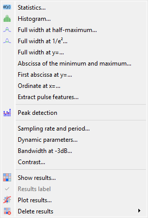
Screenshot of the “Analysis” menu.#
When the “Signal Panel” is selected, the menus and toolbars are updated to provide signal-related actions.
The “Analysis” menu allows you to perform various computations on the selected signals, such as statistics, full width at half-maximum, or full width at 1/e².
Note
In DataLab vocabulary, an “analysis” is a feature that computes a scalar result from a signal. This result is stored as metadata, and thus attached to signal. This is different from a “processing” which creates a new signal from an existing one.
Statistics#
Compute statistics on selected signal and show a summary table.
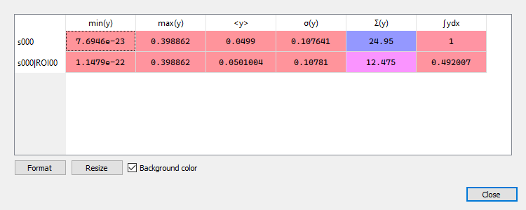
Example of statistical summary table: each row is associated to an ROI (the first row gives the statistics for the whole data).#
Histogram#
Compute histogram of selected signal and show it.
Parameters are:
Parameter |
Description |
|---|---|
Bins |
Number of bins |
Lower limit |
Lower limit of the histogram |
Upper limit |
Upper limit of the histogram |
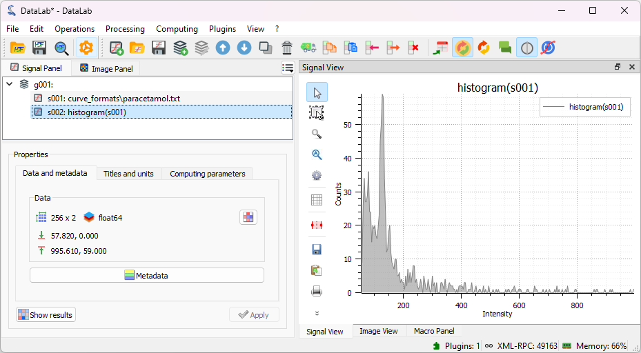
Example of histogram.#
Full width at half-maximum#
Compute the Full Width at Half-Maximum (FWHM) of selected signal, using one of the following methods:
Method |
Description |
|---|---|
Zero-crossing |
Find the zero-crossings of the signal after having centered its amplitude around zero |
Gauss |
Fit data to a Gaussian model using least-square method |
Lorentz |
Fit data to a Lorentzian model using least-square method |
Voigt |
Fit data to a Voigt model using least-square method |
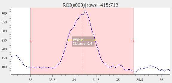
The computed result is displayed as an annotated segment.#
Full width at 1/e²#
Fit data to a Gaussian model using least-square method. Then, compute the full width at 1/e².
Note
Computed scalar results are systematically stored as metadata. Metadata is attached to signal and serialized with it when exporting current session in a HDF5 file.
Arguments of the min and max#
Compute the smallest argument of the minima and the smallest argument of the maxima of the selected signal.
Abscissa at y=…#
Compute the abscissa at a given ordinate value for the selected signal. If there is no solution, the displayed result is NaN. If there are multiple solutions, the displayed result is the smallest value.
Peak detection#
Create a new signal from semi-automatic peak detection of each selected signal.
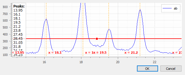
Peak detection dialog: threshold is adjustable by moving the horizontal marker, peaks are detected automatically (see vertical markers with labels indicating peak position)#
Sampling rate and period#
Compute the sampling rate and period of selected signal.
Warning
This feature assumes that the X values are regularly spaced.
Dynamic parameters#
Compute the following dynamic parameters on selected signal:
Parameter |
Description |
|---|---|
f |
Frequency (sinusoidal fit) |
ENOB |
Effective Number Of Bits |
SNR |
Signal-to-Noise Ratio |
SINAD |
Signal-to-Noise And Distortion Ratio |
THD |
Total Harmonic Distortion |
SFDR |
Spurious-Free Dynamic Range |
Bandwidth at -3 dB#
Determine the bandwidth at -3 dB by identifying the range of abscissa values where the signal remains greater than its maximum value minus 3 dB.
Warning
This feature requires that the signal is expressed in decibels (dB).
Contrast#
Compute the contrast of selected signal.
The contrast is defined as the ratio of the difference and the sum of the maximum and minimum values:
Note
This feature assumes that the signal is a profile from an image, where the contrast is meaningful. This justifies the optical definition of contrast.
Extract pulse features#
Perform comprehensive pulse analysis on selected signals, automatically extracting timing and amplitude characteristics for step and square pulse signals.
This feature provides automated pulse characterization with intelligent signal type recognition and robust parameter extraction for digital signal analysis, oscilloscope measurements, and pulse timing validation.
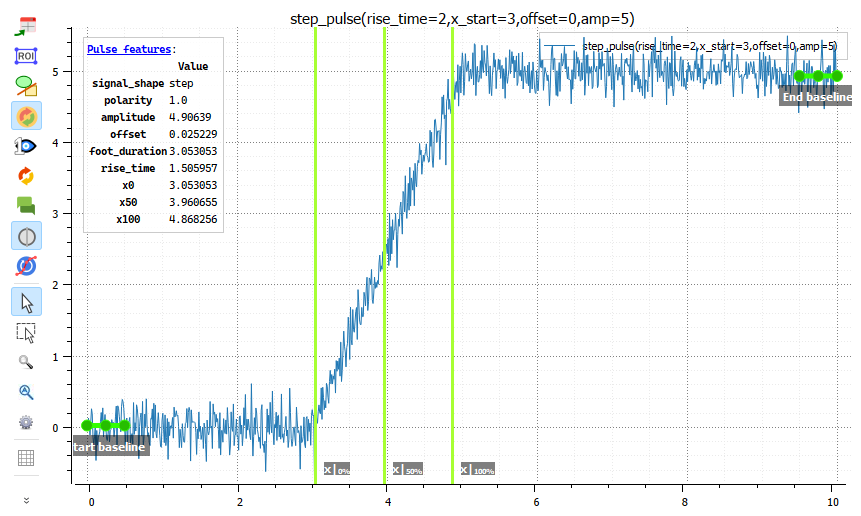
Pulse features results as displayed in the Signal View.#
Key Capabilities:
Automated signal recognition: Heuristically identifies signal type (step, square, or other) for optimal analysis
Polarity detection: Automatically determines positive/negative pulse polarity using baseline comparison
Comprehensive timing measurements: Extracts rise time, fall time, FWHM, and timing parameters at specific amplitude fractions
Baseline characterization: Analyzes start and end baseline regions for accurate feature computation
Robust algorithms: Uses advanced statistical methods with noise tolerance and error handling
Parameters:
Parameter |
Description |
|---|---|
Signal shape |
Signal type selection: Auto (automatic detection), Step, or Square |
Start baseline min |
Lower X boundary for the start (initial) baseline region |
Start baseline max |
Upper X boundary for the start (initial) baseline region |
End baseline min |
Lower X boundary for the end (final) baseline region |
End baseline max |
Upper X boundary for the end (final) baseline region |
Rise/Fall time |
Reference levels for rise/fall time measurement with predefined choices: 5%-95% (High precision), 10%-90% (IEEE standard), 20%-80% (Noisy signals), 25%-75% (Alternative) |
Extracted Features:
The analysis computes the following pulse characteristics:
Feature |
Description |
|---|---|
Signal shape |
Detected signal type (STEP, SQUARE, or OTHER) |
Polarity |
Signal polarity (+1 for positive, -1 for negative pulses) |
Amplitude |
Peak-to-peak amplitude of the pulse |
Offset |
DC offset (baseline level) |
Rise time |
Time from the lower to upper reference levels during rising edge |
Fall time |
Time from the lower to upper reference levels during falling edge (square pulses only) |
FWHM |
Full Width at Half Maximum (square pulses only) |
x50 |
Time at which signal reaches 50% of maximum amplitude |
x100 |
Time at which signal reaches 100% of maximum amplitude (plateau start) |
Foot duration |
Duration of flat region before pulse rise |
Baseline ranges |
Extracted start and end baseline boundary coordinates |
Note
Results are displayed in a comprehensive table showing all extracted parameters, and as visual annotations on the signal plot. For step signals, fall-related parameters (fall_time, fwhm) are not applicable and show as None. The feature works best with well-defined pulse signals that have clear baseline regions.
Show results#
Show the results of all analyses performed on the selected signals. This shows the same table as the one shown after having performed a computation.
Results label#
Toggle the visibility of result labels on the plot. When enabled, this checkable menu item displays result annotations (such as FWHM, peak positions, or other analysis markers) directly on the signal plot.
This option is synchronized between Signal and Image panels and persists across sessions. It is only enabled when results are available for the selected signal.
Plot results#
Plot the results of analyses performed on the selected signals, with user-defined X and Y axes (e.g. plot the FWHM as a function of the signal index).