DataLab and Spyder: a perfect match#

This tutorial demonstrates how to use Spyder to work with DataLab through a practical example, using sample algorithms and data that represent a hypothetical research or technical workflow. The goal is to illustrate how to use DataLab to test your algorithms with data and debug them when necessary.

The example is straightforward, yet it demonstrates the essential concepts of working with both DataLab and Spyder.

Note

DataLab and Spyder are complementary tools. While Spyder is a powerful development environment with interactive scientific computing capabilities, DataLab is a versatile data analysis platform that can perform a wide range of tasks, from simple data visualization to complex data analysis and processing. In other words, Spyder is a development tool, while DataLab is a data analysis tool. You can use Spyder to develop algorithms and then use DataLab to analyze data with those algorithms.

Basic concepts#

In the context of your research or technical work, we assume that you are developing software to process data (signals or images). This software may be a stand-alone application, a library for use in other applications, or even a simple script to run from the command line. In any case, you will need to follow a development process that typically includes the following steps:

Prototype the algorithm in a development environment such as Spyder.
Develop the algorithm in a development environment such as Spyder.
Test the algorithm with data.
Debug the algorithm if necessary.
Repeat steps 2 and 3 until the algorithm works as expected.
Use the algorithm in your application.

Note

DataLab can help you with step 0 because it provides all the processing primitives you need to prototype your algorithm: you can load data, visualize it, and perform basic processing operations. We won’t cover this step in the following sections since the DataLab documentation already provides extensive information about it.

In this tutorial, we will see how to use DataLab to perform steps 2 and 3. We assume that you have already prototyped (preferably in DataLab!) and developed your algorithm in Spyder. Now, you want to test it with data, but without leaving Spyder because you may need to modify your algorithm and re-test it. Besides, your workflow is already set up in Spyder and you don’t want to change it.

Note

This tutorial assumes that you have already installed DataLab and started it. If you haven’t done so yet, please refer to the Installation section of the documentation.

Additionally, we assume that you have already installed Spyder and started it. If you haven’t done so yet, please refer to the Spyder documentation. Note that you don’t need to install DataLab in the same environment as Spyder: that’s the whole point of DataLab—it is a stand-alone application that can be used from any environment. For this tutorial, you only need to install the Sigima package (pip install sigima) in the same environment as Spyder.

Testing your algorithm with DataLab#

Let’s assume that you have developed algorithms in the my_work module of your project. You have already prototyped them in DataLab and developed them in Spyder by writing functions that take data as input and return processed data as output. Now, you want to test these algorithms with data.

To test these algorithms, you have written two functions in the my_work module:

test_my_1d_algorithm: this function returns 1D data that will allow you to validate your first algorithm, which processes 1D data.
test_my_2d_algorithm: this function returns 2D data that will allow you to validate your second algorithm, which processes 2D data.

You can now use DataLab to visualize the data returned by these functions directly from Spyder:

First, start both DataLab and Spyder.
Remember that DataLab is a stand-alone application that can be used from any environment, so you don’t need to install it in the same environment as Spyder because the connection between these two applications is established through a communication protocol.

Here is how to do it:

# %% Connecting to DataLab current session

from sigima.client import SimpleRemoteProxy

proxy = SimpleRemoteProxy()
proxy.connect()

# %% Visualizing 1D data from my work

from my_work import test_my_1d_algorithm

x, y = test_my_1d_algorithm()  # Here is all my research/technical work!
proxy.add_signal("My 1D result data", x, y)  # Let's visualize it in DataLab
proxy.compute_wiener()  # Denoise the signal using the Wiener filter


# %% Visualizing 2D data from my work

from my_work import test_my_2d_algorithm

z = test_my_2d_algorithm()[1]  # Here is all my research/technical work!
proxy.add_image("My 2D result data", z)  # Let's visualize it in DataLab

If we execute the first two cells, we will see the following output in the Spyder console:

Python 3.11.5 (tags/v3.11.5:cce6ba9, Aug 24 2023, 14:38:34) [MSC v.1936 64 bit (AMD64)]
Type "copyright", "credits" or "license" for more information.

IPython 8.15.0 -- An enhanced Interactive Python.

In [1]: runcell('Connecting to DataLab current session', 'my_work_test_with_datalab.py')
Connecting to DataLab XML-RPC server...OK (port: 54577)

In [2]: runcell('Visualizing 1D data from my work', 'my_work_test_with_datalab.py')
Out[2]: True

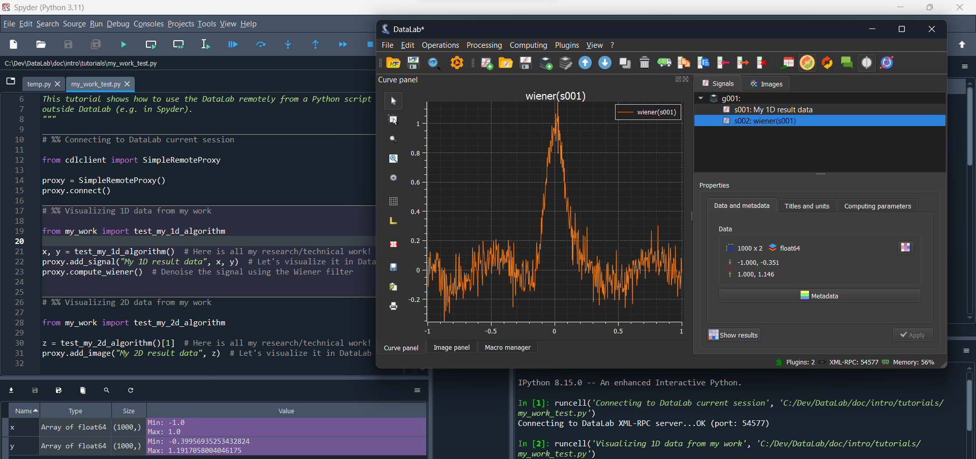
../../_images/015.png — In this screenshot, we can see the result of evaluating the first two cells: the first cell connects to DataLab, and the second cell visualizes the 1D data returned by the `test_my_1d_algorithm` function.#

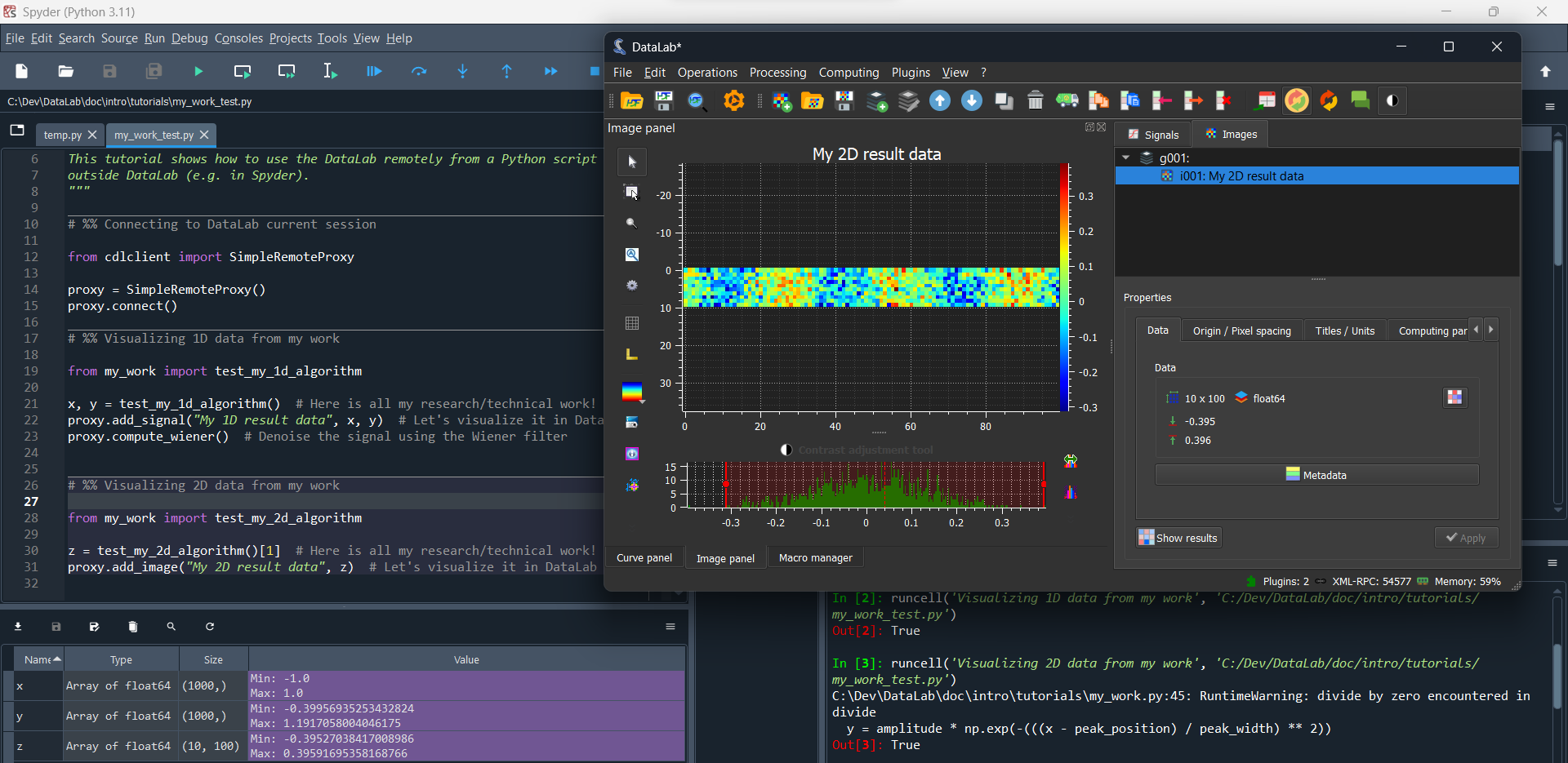
../../_images/025.png — In this screenshot, we can see the result of evaluating the third cell: the `test_my_2d_algorithm` function returns a 2D array, which we can visualize directly in DataLab.#

Debugging your algorithm with DataLab#

Now that you have tested your algorithms with data, you may want to debug them if necessary. To do so, you can combine the Spyder debugging capabilities with DataLab.

Here is the code of the sample algorithm that we want to debug, in which we have introduced an optional debug_with_datalab parameter that—if set to True— will create a proxy object allowing step-by-step visualization of the data in DataLab:

def generate_2d_data(
    num_lines: int = 10,
    noise_std: float = 0.1,
    x_min: float = -1,
    x_max: float = 1,
    num_points: int = 100,
    debug_with_datalab: bool = False,
) -> tuple[np.ndarray, np.ndarray]:
    """Generate 2D data that can be used in the tutorials to represent some results.

    Args:
        num_lines: Number of lines in the generated data, by default 10.
        noise_std: Standard deviation of the noise, by default 0.1.
        x_min: Minimum value of the x axis, by default -1.
        x_max: Maximum value of the x axis, by default 1.
        num_points: Number of points in the generated data, by default 100.
        debug_with_datalab: Whether to use the DataLab to debug the function,
         by default False.

    Returns:
        Generated data (x, y; where y is a 2D array and x is a 1D array).
    """
    proxy = None
    if debug_with_datalab:
        proxy = SimpleRemoteProxy()
        proxy.connect()
    z = np.zeros((num_lines, num_points))
    for i in range(num_lines):
        amplitude = 0.1 * i**2
        peak_position = 0.5 * i**2
        peak_width = 0.1 * i**2
        x, y = generate_1d_data(
            amplitude,
            peak_position,
            peak_width,
            relaxation_oscillations=True,
            noise=True,
            noise_std=noise_std,
            x_min=x_min,
            x_max=x_max,
            num_points=num_points,
        )
        z[i] = y
        if proxy is not None:
            proxy.add_signal(f"Line {i}", x, y)
    return x, z

The corresponding test_my_2d_algorithm function also has an optional debug_with_datalab parameter that is simply passed to the generate_2d_data function.

Now, we can use Spyder to debug the test_my_2d_algorithm function:

# %% Debugging my work with DataLab

from my_work import generate_2d_data

x, z = generate_2d_data(debug_with_datalab=True)

In this simple example, the algorithm iterates 10 times and generates a 1D array at each iteration. Each 1D array is then stacked into a 2D array that is returned by the generate_2d_data function. With the debug_with_datalab parameter set to True, we can visualize each 1D array in DataLab: that way, we can verify that the algorithm is working as expected.

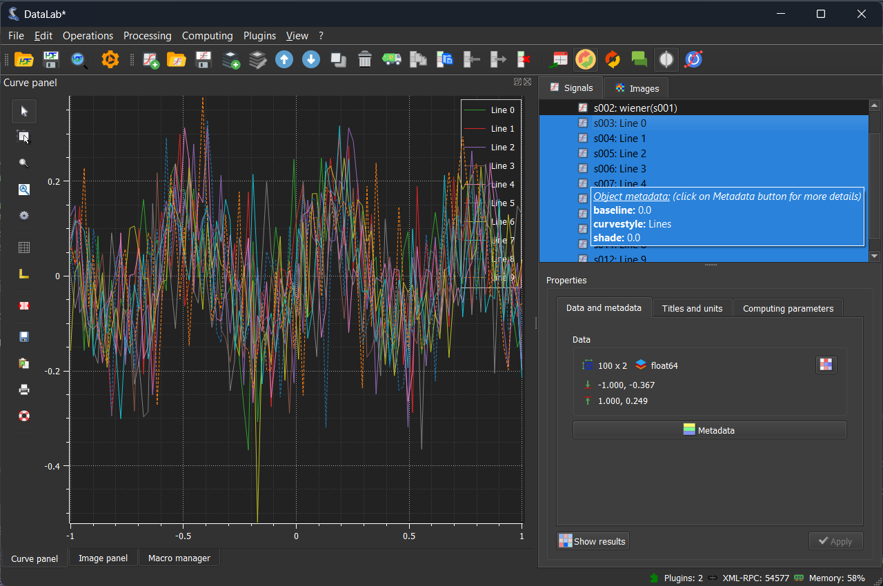
../../_images/035.png — In this screenshot, we can see the result of evaluating the first cell: the `test_my_2d_algorithm` function is called with the `debug_with_datalab` parameter set to `True`: 10 1D arrays are generated and visualized in DataLab.#

Note

If we had executed the script using the Spyder debugger and set a breakpoint in the generate_2d_data function, we would have seen the generated 1D arrays in DataLab at each iteration. Since DataLab runs in a separate process, we would have been able to interact with the data in DataLab while the algorithm is paused in Spyder.