Detecting blobs on an image

This example shows how to detect blobs on an image with DataLab, and also covers other features such as the plugin system:

• Add a new plugin to DataLab

• Denoise an image

• Detect blobs on an image

• Save the workspace to a file

First, we open DataLab, and open the settings dialog (using “File > Settings…”, or the icon in the toolbar).

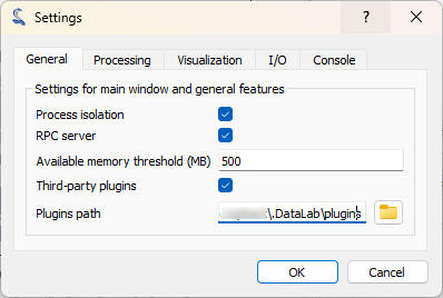
In the “General” tab, we can see the “Plugins path” field. This is the path where DataLab will look for plugins. We can add a new plugin by copying/pasting the plugin file in this directory.

See also

The plugin system is described in the Plugins section.

Let’s add the datalab_example_imageproc.py plugin to DataLab (this is an example plugin that is shipped with DataLab source package, or may be downloaded from here).

If we close and reopen DataLab, we can see that the plugin is now available in the “Plugins” menu: there is a new “Extract blobs (example)” entry.

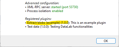
The “About DataLab” dialog shows the list of available plugins.

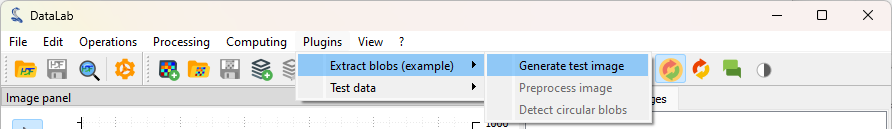
Let’s click on “Extract blobs (example) > Generate test image”

Note

DataLab menus change between images and signals. To be able to see the “Extract blobs (example)” menu, make sure that the “Images” panel is selected (click on the “Images” tab on the left).

A pop-up dialog appears, asking for the parameters of the test image to generate (the size of the image and its title). We can just keep the default parameters and click on “OK”.

For information, the image is generated by the plugin using the following code:

def generate_test_image(self) -> None:
    """Generate test image"""
    newparam = self.edit_new_image_parameters(
        title="Test image", hide_dtype=True, shape=(2048, 2048)
    )
    if newparam is not None:
        # Create a NumPy array:
        shape = (newparam.height, newparam.width)
        arr = np.random.normal(10000, 1000, shape)
        for _ in range(10):
            row = np.random.randint(0, shape[0])
            col = np.random.randint(0, shape[1])
            rr, cc = skimage.draw.disk((row, col), min(shape) // 50, shape=shape)
            arr[rr, cc] -= np.random.randint(5000, 6000)
        center = (shape[0] // 2,) * 2
        rr, cc = skimage.draw.disk(center, min(shape) // 10, shape=shape)
        arr[rr, cc] -= np.random.randint(5000, 8000)
        data = np.clip(arr, 0, 65535).astype(np.uint16)

        # Create a new image object and add it to the image panel
        obj = sigima.objects.create_image(
            newparam.title, data, units=("mm", "mm", "lsb")
        )
        self.proxy.add_object(obj)

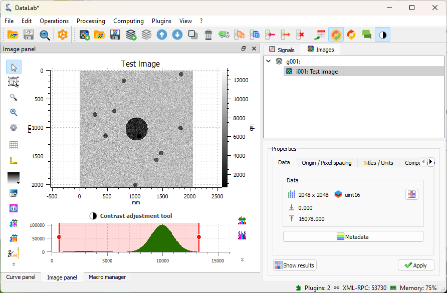
The plugin has generated a test image, and added it to the “Images” panel. The image shows a few blobs, with a central bigger disk, and a noisy background.

The plugin has other features, such as denoising the image, and detecting blobs on the image, but we won’t cover them here: we will instead use the DataLab native features to achieve, manually, the same operations as the plugin.

The image is a bit noisy, and also quite large. In addition, the blobs are large with respect to the pixel size.

To reduce the noise there are several functions available in DataLab. Due to the considerations we just made, we can consider that a binning would reduce the noise without losing the information we look for. Let’s apply a binning to the image by a factor of 2 on both axes. This will reduce the image size by a factor of 4, and the noise standard deviation by a factor of 2. Choosing to change the pixel size accordingly will keep the blob size constant in the previous unit (in this case, pixels, but in a real application we can calibrate them to respect a real physical size).

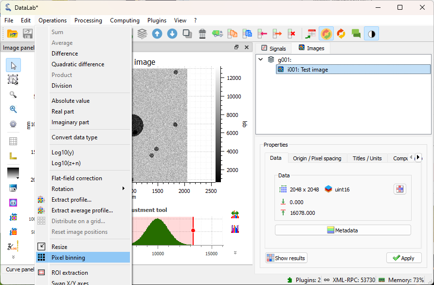
Click on “Operations > Pixel binning”.

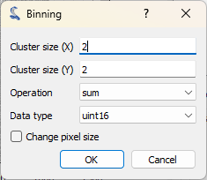
The “Binning” dialog opens, with several options. Set the binning factor to 2 for both axes, select the “change pixel size” case and click on “OK”.

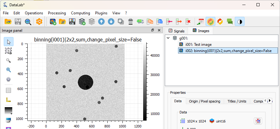
The binned image is added to the “Images” panel. It is now easier to see the blobs (even if they were already quite visible on the original image: this is just an example), and the image will be faster to process.

A different approach we can take is to apply a moving median filter, to reduce the importance of the spikes. We do it with a window of 5; of course in practice different window sizes can be tested to find a good compromise between noise reduction and resolution. Let’s see how to do that.

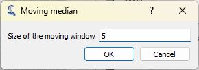
Click on “Processing > Noise reduction > Moving median” entry, and set the window size to 5.

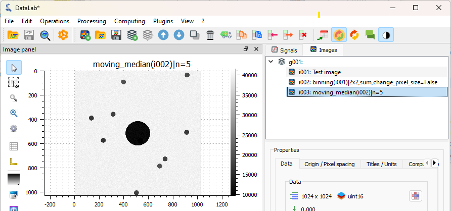
The filtered image is added to the “Images” panel. Denoising is quite efficient.

Now, we can be satisfied with our denoising: it is visible that the noise is smaller. We can thus move to the following step: detect the blobs on the image. To do that, we can use the “Blob detection” function available in the “Analysis” menu. Different algorithms are available, here we will use the OpenCV one.

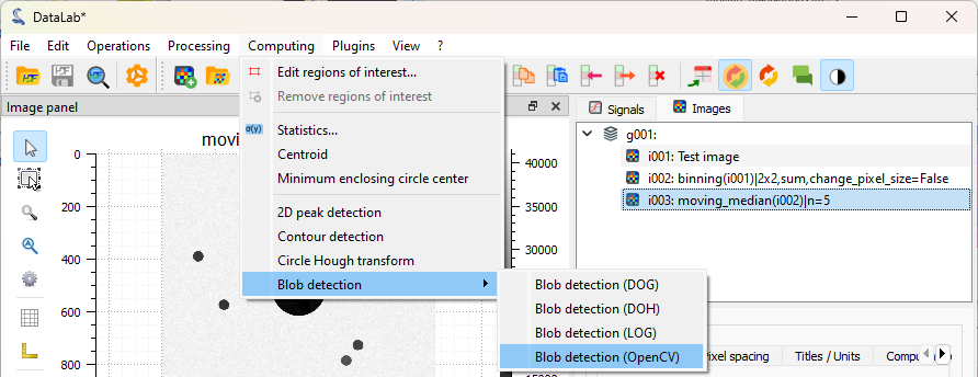
Click on “Analysis > Blob detection > Blob detection (OpenCV)”.

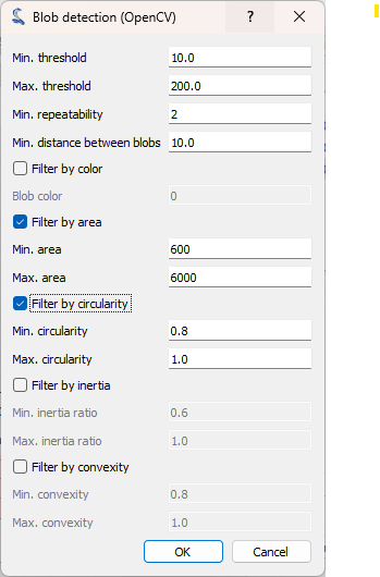
The “Blob detection (OpenCV)” dialog opens. Set the parameters as shown on the screenshot, and click on “OK”.

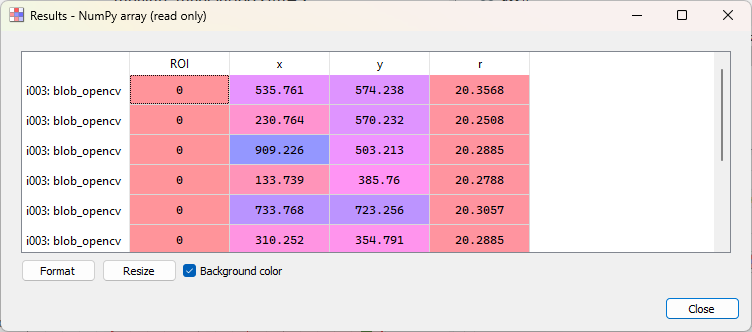
The “Results” dialog opens, showing the detected blobs: one line per blob, with the blob coordinates and radius.

Note

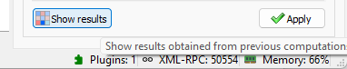
If you want to show the analysis results again, you can select the “Show results” entry in the “Analysis” menu, or the “Results” button, in the property panel below the image list:

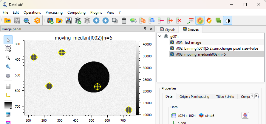
The detected blobs are also added to the image metadata, and can be seen in the visualization panel on the right.

Finally, we can save the workspace to a file. The workspace contains all the images that were loaded in DataLab, as well as the processing results. It also contains the visualization settings (colormaps, contrast, etc.), the metadata, and the annotations. To save the workspace, click on “File > Save to HDF5 file…”, or the button in the toolbar.

If you want to load the workspace again, you can use the “File > Open HDF5 file…” (or the button in the toolbar) to load the whole workspace, or the “File > Browse HDF5 file…” (or the button in the toolbar) to load only a selection of data sets from the workspace.